StimPlan™ can be used for real time data acquisition in several ways, but all methods require that the data be “converted” by another computer. That is, StimPlan™ does not directly connect to pressure transducers, densitometers, etc. This discussion here is dived into two parts – where the data might be coming from, and how to get this data into StimPlan™.

Data Sources

In order to import “Real Time” data into StimPlan™, the data must reside in an ASCII file on the same computer (or a connected network) where StimPlan™ is installed and running. The source of this data is of no concern to StimPlan™, nor is the data frequency, nor how often data is added to this file. Some examples might include:

Internet:

Many treatments are monitored remotely, using Internet facilities of the pumping company. These facilities allow you to view plots in real time, and also have a capability to output the data directly to an ASCII file on the monitoring computer. Thus, the Internet site is writing data into a text file one line at a time. For example, this file might look like

09:12:22	4212.12	24.33	6.17	4.71	20.01, etc.
09:12:23	4218.34	24.21	6.24	4.84	20.12, etc.

and, of course, you will need to know (in advance) what each column of data represents. Every “N” seconds, StimPlan™ will then sample this file for new data, and if new data is present it will be imported. Note that in this example, data appears to be arriving at one data point per second, but say that StimPlan™ is set to check this file every 20 seconds. This is not a problem; StimPlan™ simply imports 20 data points at a time.

COMM Port:

For direct computer-to-computer data transfer, currently the most common method is via a “COMM:” or “Serial:” port. On the back of the computer, such a port will look like the red circled 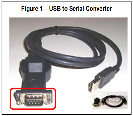connection in Figure 1. A male connection with 9 pins (a DB9 connector). Serial data transfer for accessories (printers, etc.) is less used to day, so some computers donot have Serial ports. In that case, a USB to Serial Converter (along with the appropriate driver CD) will be needed to convert a USB port into a Serial port.

A DB9 Serial Data Transfer cable (sometimes called a “Null Modem” cable) is then required. This cable will have a DB9 female connector on each end (as compared to the male connector seen in the figure), and this is what connects the two computers. The sending computer will then send data out the serial port one character at a time, and the receiving computer must use some software to convert this continuous serial stream of data back into a file. This can be done with commercial software. For one example, the HyperTerm program (a Windows accessory) can be used for this. HyperTerm can receive the data, print it to the screen for visual checking, and then write the data

to an ASCII file line at a time. Details of this can be found in the Windows Help. Within StimPlan™, there is also supplied utility “CommWatch”.

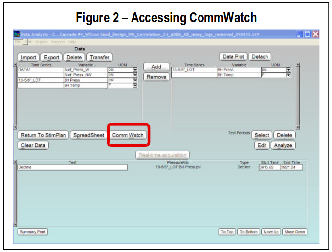
CommWatch is accessed from the Pressure Analysis dialog pictured in Figure 2. To begin a direct computer-to-computer data acquisition, this would then be the first step, run CommWatch. This data acquisition program then opens to the dialog seen in Figure 3.

On opening, you may first get a message
     “Remove older log files
     C:\abcde\HyperWatch*.log”.

These are log files from previous data acquisitions; the answer here is virtually always “Yes”.

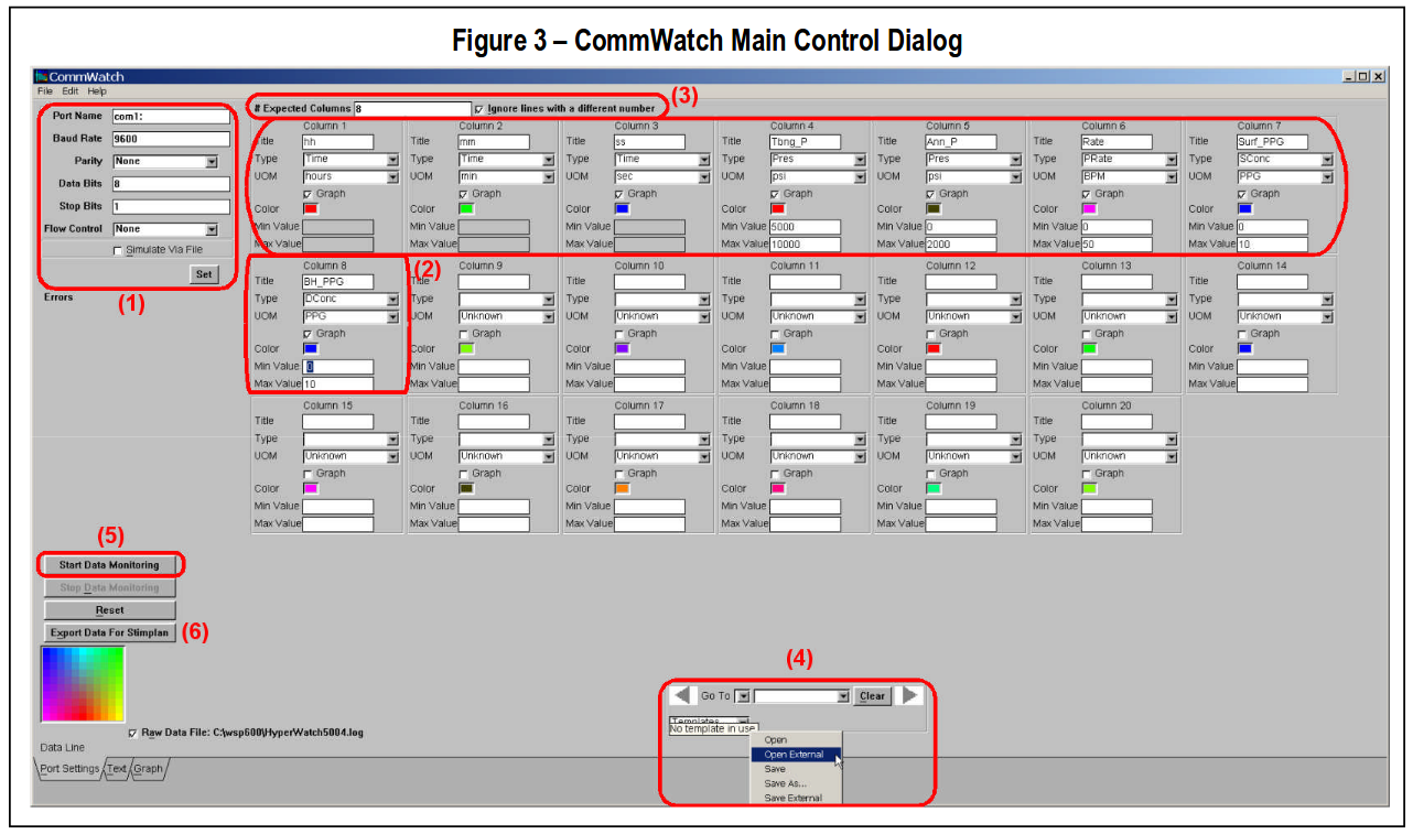
• Settings for Serial (COMM) Port (1) – The first step is to set the communications settings for the receiving serial port (top-left). If the serial data port is built into the computer, this is almost always “COMM1:”. If this is not the case, or if a USB Serial Converter is used, Window’s Device Manager can be used to locate the active “COMMx:” port. The remaining 5 settings must be supplied by the “sender”, though the default values (9600, None, 8, 1, None) are very common. After the desired inputs are specified, click “Set” to apply these settings.

• Identify Incoming Data (2) – For each valid line of data, every data point must be identified, or at least (as seen above), the first 8 data on each line must be identified. That is, each line of valid data could have data values of “Breaker Conc”, Fluid Viscosity”, etc. and these data points 9 & 10 can be ignored if not desired. However, unlike importing data into StimPlan™, you cannot parse the incoming serial data transfer and read the first two data points, skip the third, read the fourth, etc. The number of data to be read from each line is then required to be input above
(3) . Optionally, a choice can be made to reject the entire line of data for any line with more than 8 numbers, or to accept such lines of data and only read the first 8 values. Most often, “Ignore Lines” is selected to minimize chances of “noise” contaminating a data stream.
     Finally, note the “Min”/”Max” values. These only refer to the expected range of the data, or the range that will be plotted in the “Graph” tab (at bottom). This produces a scrolling Variable vs. Time Plot of all recorded data, as fast as the data is received.

• Templates (4) – If desired, all of these settings can be saved as “Templates” for future use. In this case, no template has been imported so no template is currently in use. Thus, one could: “Save As” – This saves the setting in YOUR graph preferences file. This is then recalled using the “Open” command, but is not readily available for other users.
“Save External” – This saves the setting in an external ASCII file that can readily be shared. The actual settings are then saved/opened using the standard Window’s file dialogs.

• Start Data Monitoring (5) – Selecting “Start Data Monitoring” causes CommWatch to start reading the serial port, if data is received, it is written to the “Text” tab (see below) and plotted in the “Graph” tab. It is also stored locally (within CommWatch) for later transfer to StimPlan™. Note that ALL data received after “Start Data Monitoring” is saved within CommWatch until “Reset” is selected or the program is closed.

• Export Data (6) – When ready, “Export Data for StimPlan™” will create a file (using the normal Window’s file dialog), and will write all of the data recorded since “Start” was selected into that file. Data will then be added to that file once/second, or once per two seconds, or whatever. As fast as data is received – it is added to this ASCII file. By default this has a “.TPR” (Time. Pressure/Rate) extension, and if that extension is maintained, the data file will be written in such a manner that StimPlan™ will automatically recognize the data and know that time has a format of HH:MM:SS in columns 1, 2, & 3, etc.

When done, the “formal” path to stop Data Acquisition would be to choose “Stop Real Time Acquisition”, then “Alt-Tab” to CommWatch and choose “Reset”, and then finally exit CommWatch. Alternatively, one can simply exit CommWatch.

CommWatch Displays:

There are two data displays in CommWatch. First the “Text” tab (at the bottom-left of the 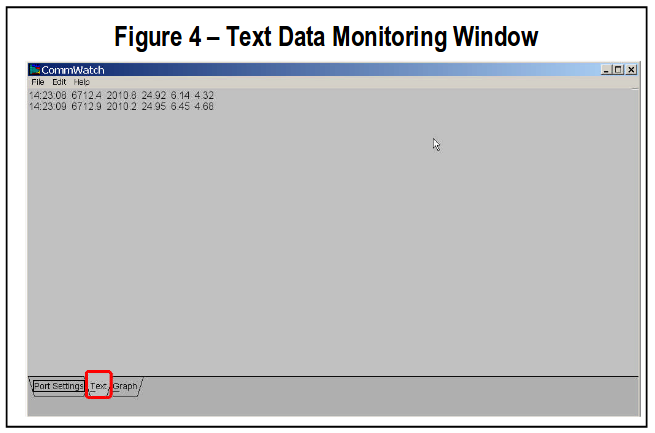window). If “Text” is selected, the text monitoring window opens as seen in Figure 4. As lines of data are then received via the Serial Data Port, they will be printed and will scroll down on this window.

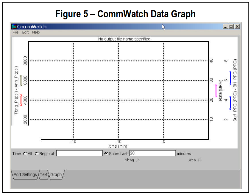
The second display is the “Graph” tab (bottom-left of window). As seen in Figure 5, this produces a scrolling display of the data is it is received. In this example, the plot is set to scroll with time always displaying the last 20 minutes of data. This graph is controlled by choices for each variable in the CommWatch main window.

Real-Time Data Import – StimPlan™

Some mechanism is creating an ASCII data file with incoming real-time data. This could be an In-ternet portal of the pumping company, via a serial data port & CommWatch, or using Window’s HyperTerm and receiving data via a phone modem. To StimPlan™, it does not matter how this ASCII file is being created, how often 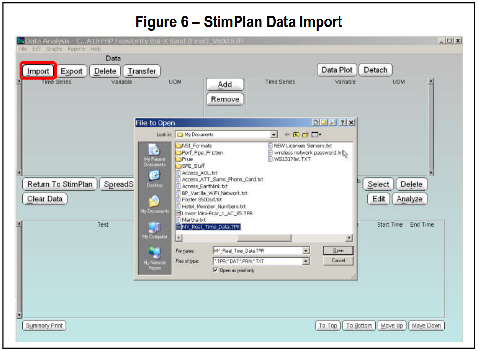is data being added, or even if this is a “Real-Time” acquisition or a postfrac import. All procedures within StimPlan™ are basically the same for realtime data import/analysis/simulation as for a post-frac data import/analysis/..... The only difference is small changes in the Data Import process.

     After opening the Pressure/Rate Analysis Module from the main StimPlan™ window, the first step is to select Import (top-left) (Figure 6). The desired file is then selected using normal Window’s file dialogs. This opens the Import Analysis Data dialog as seen in Figure 7.

     If this is a CommWatch generated TPR file, then the column headers for the 8 columns of data will be automatically completed. Otherwise, these must be completed manually describing a title, Data Type, and UOM for each column. This is identical to normal StimPlan™ data imports for postfrac analysis. The differences lie in the two inputs near the bottom of the dialog:

• Real Time Acquisition
• Sample Interval (seconds)

     For a real-time acquisition, this option is “selected”. Then, a sample interval must be specified. If recording pre-frac test data real-time, this should normally be set to something like 10 or 20 seconds (this allows reasonable analysis time between bursts of data acquisition). However, NO DATA IS LOST. If the incoming data is once/second, and this Sample Interval is set for 10 seconds – that simply means 10 new data points will be imported each time StimPlan™ accesses this file. StimPlan™ is then used as normal to analysis pre-frac data, history match recorded pressure data, develop a final design, etc. In the background the data is being imported every 10 seconds, but that in now way changes how StimPlan™ is used.

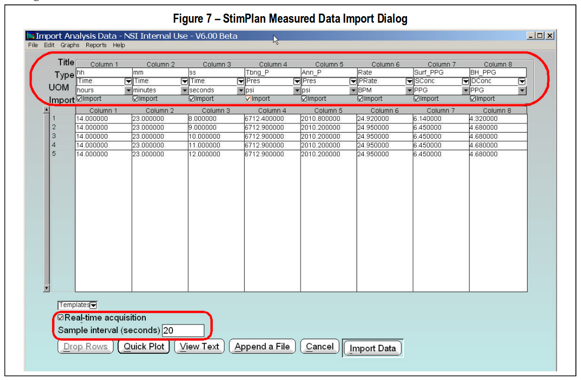
If real-time data is simply being monitored, the sample interval can be set to 1 or 2 seconds. Also, this can be changed later from within StimPlan™ (in the Pressure/Rate Analysis module).

Real-Time Data Display – StimPlan™

Within StimPlan™, Real-Time data displays 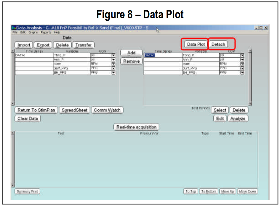can be created using the “Data Plot” (Fig-ure 8). The desired data is selected in the “Data” area on the left, and then “Added” to the Data Plot. Selecting “Data Plot” then opens a data vs. time graph. This is seen in Figure 9 below, and the graph updates as new data is received. NOTE, however, that once the data exceeds the current maximum time, one must either:

• Right-click and use graph Settings to manually change the time scale, or
• “OK” to exit the Data Plot, and then re-enter. This forces a new auto-scaling.

The example below shows an example where data acquisition is just starting.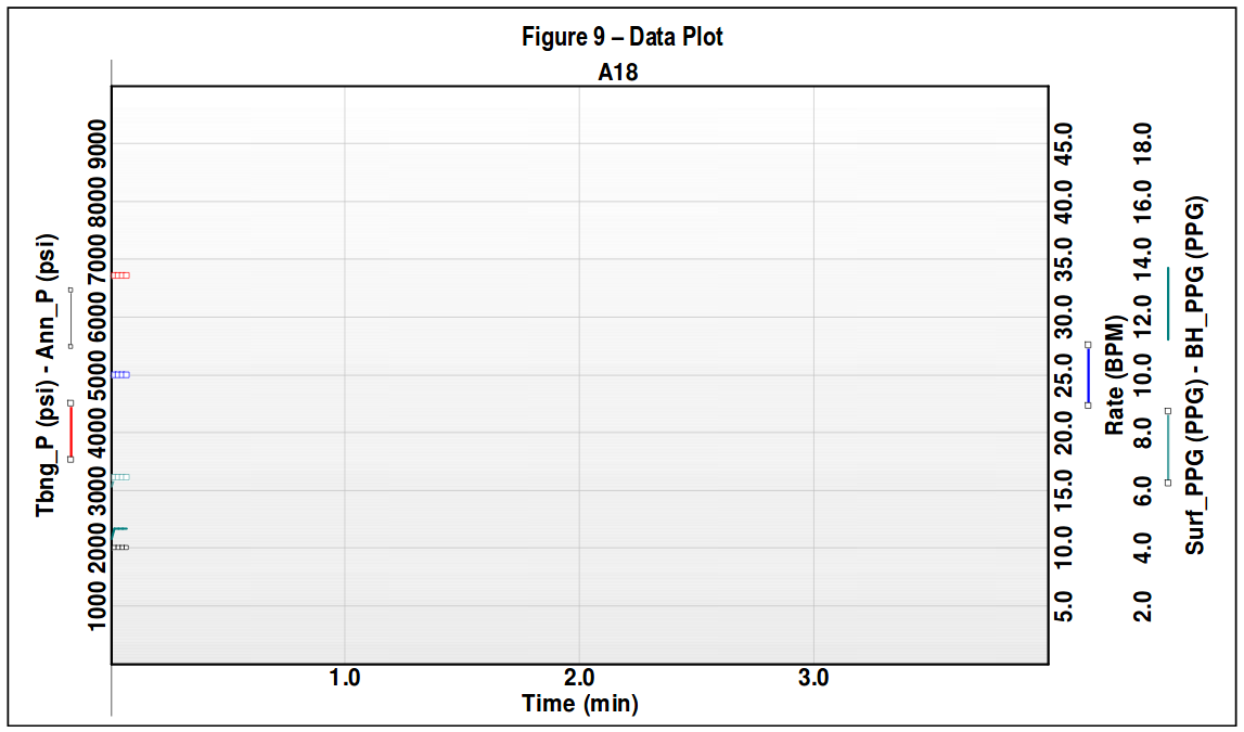

Detached Plots

Multiple graph windows can be creating using 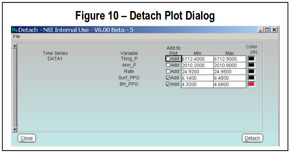“Detach” (see Figure 8). This opens the dialog in Figure 10. In this example the two proppant concentration variables have been selected to be displayed in a separate plot.